Combining R & Observable javascript with Quarto

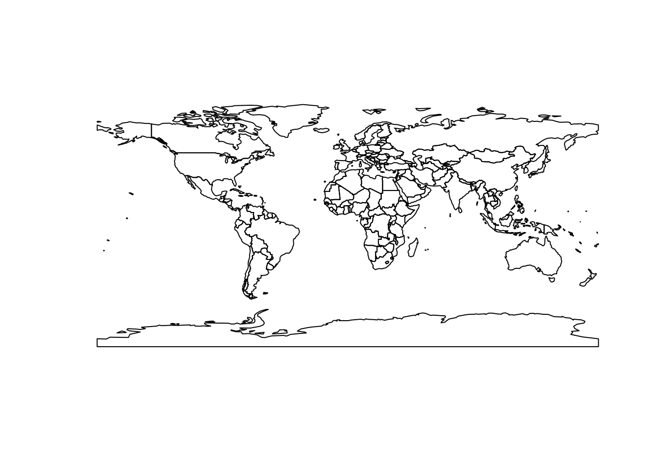
Quarto is an open-source scientific and technical publishing system built on Pandoc. It allows to create dynamic content with Python, R, Julia, and Observable. In this document, I show how it is now possible to combine a an analysis written in R and a visualization written in Observable javascript.

1. Data handling & analysis In R

With the sf library, we import a gpkg file containing world countries and display it.

Code

library("sf")
countries <- st_read("data/countries.gpkg", quiet = T)
plot(st_geometry(countries))

We now import a statistical file in csv format containing the population and wealth of the countries of the world.

Code

data <- read.csv("data/stat.csv")
head(data)

   id                 name  region      pop          gdp    gdppc year
1 AFG          Afghanistan    Asia 38928341  19807067268   508.81 2020
2 AGO               Angola  Africa 32866268  62306913444  1895.77 2020
3 ALB              Albania  Europe  2837743  14799615097  5215.28 2020
4 AND              Andorra  Europe    77146   3155065488 40897.33 2019
5 ARE United Arab Emirates    Asia  9770526 421142267937 43103.34 2019
6 ARG            Argentina America 45376763 383066977654  8441.92 2020

Then, we perform a join between the basemap and the statistical data by matching the identical codes.

Code

world = merge(countries, data, by.x = "ISO3", by.y = "id")

To create a map in Observable, we first need to convert this data set to geojson format. To do this, we use the geojsonsf library. Then, the ojs_define() instruction allows to define this variable within ojs cells. To learn more about passing variables from R to Ojs, you can visit this page.

Code

library(geojsonsf)
ojs_define(world_str = sf_geojson(world))

NB: Note that here we have passed the variable as a string and not actually as an object. That’s why we called it world_str.

2. Geoviz in Observable Javascript (ojs)

The first thing to do here is to transform our string into a real object. To do this, we use the javascript statement JSON.parse.

Code

world = JSON.parse(world_str)

We display the attribute table to check that everything is ok.

Code

Inputs.table(world.features.map((d) => d.properties))

We import the javascript libraries needed for mapping. Here d3-geo-projection@4 to have access to additional mapping projections and bertinjs for the mapping itself.

Code

d3 = require("d3@7", "d3-geo-projection@4")
bertin = require('bertin@0.9.16')

We define some elements for the interaction with the user.

Code

viewof val = Inputs.radio(["pop", "gdp"], {
  label: "Data to be displayed",
  value: "pop"
})
viewof step = Inputs.range([10, 50], {
  label: "step",
  step: 1,
  value: 15
})
viewof k = Inputs.range([5, 30], {
  label: "Radius of the largest circle",
  step: 1,
  value: 15
})
viewof dorling = Inputs.toggle({ label: "Avoid overlap (dorling)" })

Then we create a thematic interactive map with bertinjs. For more information about bertinjs, see this and that.

Code

bertin.draw({
  params: { projection: d3.geoBertin1953() },
  layers: [
    {
      type: "header",
      text:
        (val == "pop" ? "World population" : "World GDP") + ` (step = ${step})`,
      fill: "#cf429d"
    },
    {
      type: "regularbubble",
      geojson: world,
      step: step,
      values: val,
      k: k,
      fill: "#cf429d",
      tooltip: [
        "$NAMEen",
        "",
        "country value",
        `$${val}`,
        "",
        "dot value",
        "$___value" // ___value is the name of the computed field with the value of the point
      ],
      dorling: dorling
    },
    { geojson: world, fill: "white", fillOpacity: 0.3, stroke: "none" },
    { type: "graticule" },
    { type: "outline" }
  ]
})