Quarto: ojs_define & transpose

In this document, we show how it is possible to pass a variable from R to Observable. We deal with 3 cases:

• a simple variable
• a data frame
• a spatial data frame (sf)

1 - a simple variable

{r}

Here we have a variable myvar which is 12.

myvar = 12

The ojs_define instruction simply makes this variable accessible in Observable

ojs_define(myvar)

{ojs}

myvar

12

1 - a dataframe

{r}

In this second case, we import a csv file.

data <- read.csv("data/stat.csv")

As before, we use ojs_define to make this variable accessible in Observable. We rename this variable to newdata.

ojs_define(newdata = data)

{ojs}

Warning, if we visualize this data table in Observable directly, we realize that it does not really have the expected form.

newdata

Object {id: Array(209), name: Array(209), region: Array(209), pop: Array(209), gdp: Array(209), gdppc: Array(209), year: Array(209)}

Thankfully, the transpose instruction allows you to convert the table to the correct format.

data = transpose(newdata)
data

data = Array(209) [Object, Object, Object, Object, Object, Object, Object, Object, Object, Object, Object, Object, Object, Object, Object, Object, Object, Object, Object, Object, …]

Array(209) [Object, Object, Object, Object, Object, Object, Object, Object, Object, Object, Object, Object, Object, Object, Object, Object, Object, Object, Object, Object, …]

Inputs.table(data)

	id	name	region	pop	gdp	gdppc	year
	AFG	Afghanistan	Asia	38,928,341	19,807,067,268	508.81	2,020
	AGO	Angola	Africa	32,866,268	62,306,913,444	1,895.77	2,020
	ALB	Albania	Europe	2,837,743	14,799,615,097	5,215.28	2,020
	AND	Andorra	Europe	77,146	3,155,065,488	40,897.33	2,019
	ARE	United Arab Emirates	Asia	9,770,526	421,142,267,937	43,103.34	2,019
	ARG	Argentina	America	45,376,763	383,066,977,654	8,441.92	2,020
	ARM	Armenia	Asia	2,963,234	12,645,459,214	4,267.45	2,020
	ATA	Antarctica	Antarctica
	ATG	Antigua and Barbuda	America	97,928	1,415,059,259	14,450	2,020
	AUS	Australia	Oceania	25,687,041	1,330,900,925,057	51,812.15	2,020
	AUT	Austria	Europe	8,917,205	430,947,393,758	48,327.63	2,020
	AZE	Azerbaijan	Asia	10,110,116	42,607,176,471	4,214.31	2,020
	BDI	Burundi	Africa	11,890,781	3,258,187,233	274.01	2,020
	BEL	Belgium	Europe	11,555,997	515,332,499,628	44,594.38	2,020
	BEN	Benin	Africa	12,123,198	15,651,545,209	1,291.04	2,020
	BFA	Burkina Faso	Africa	20,903,278	17,369,059,295	830.93	2,020
	BGD	Bangladesh	Asia	164,689,383	324,239,176,765	1,968.79	2,020
	BGR	Bulgaria	Europe	6,927,288	69,105,101,090	9,975.78	2,020
	BHR	Bahrain	Asia	1,641,164	38,474,521,277	23,443.43	2,019
	BHS	Bahamas	America	393,248	11,250,000,000	28,607.9	2,020
	BIH	Bosnia and Herzegovina	Europe	3,280,815	19,788,422,248	6,031.56	2,020
	BLR	Belarus	Europe	9,398,861	60,258,239,056	6,411.23	2,020
	BLZ	Belize	America	397,621	1,763,696,119	4,435.62	2,020

3 - a spatial data frame (sf)

{r}

In this third case, we import a geopakage thanks to the library sf, containing the countries of the world.

library("sf")
countries <- st_read("data/countries.gpkg", quiet = T)
plot(st_geometry(countries))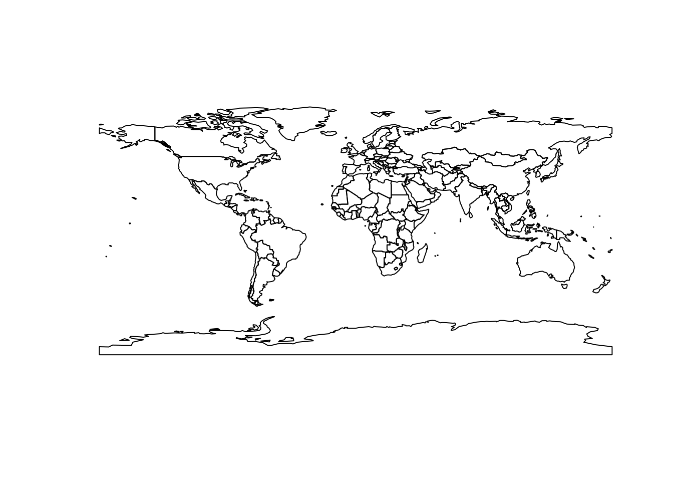

To create a map in Observable, we first need to convert this data set to geojson format. To do this, we use the geojsonsf library. Then, the ojs_define() instruction allows to define this variable within ojs cells.

library("geojsonsf")
ojs_define(geo = sf_geojson(countries))

{ojs}

Note that with ojs_define, we have passed the variable geo as a string and not actually as an object.

geo.substr(1, 300)

`"type":"FeatureCollection","features":[{"type":"Feature","properties":{"ISO3":"GNQ","NAMEen":"Equatorial Guinea","NAMEfr":"Guinée-Équatoriale"},"geometry":{"type":"MultiPolygon","coordinates":[[[[11.322078491,2.165760396],[11.336341187,0.999164937],[9.8043711812,0.9983539399],[9.3466903,1.181708075]`

The first thing to do here is to transform our string into a real object. To do this, we use the javascript statement JSON.parse.

countries = JSON.parse(geo) 
countries

countries = Object {type: "FeatureCollection", features: Array(209)}

Object {type: "FeatureCollection", features: Array(209)}

Now everything is ok to make a map in Observable. See more here.

bertin = import('https://cdn.skypack.dev/bertin@0.9.12')
bertin.draw({
  layers: [
    {
      geojson: countries,
      tooltip:["$ISO3","$NAMEen"]
    }
    ]
})

4 - Another solution

Another way to pass variables and data from R to Observable is to save and then import data.

{r}

As before, we import a geopackage in R with sf.

countries <- st_read("data/countries.gpkg", quiet = T)

Then we convert it to geojson and save it in the data directory.

write(sf_geojson(countries), "data/world.geojson")

{ojs}

In observable, we just have to import this data file in geojson (or other) format.

world = FileAttachment("data/world.geojson").json()

world = Object {type: "FeatureCollection", features: Array(209)}

Let’s take a look at it!

bertin.quickdraw(world)

That’s all folks!