library(readxl)
library(sf)
library(packcircles)
library(magick)Le cartogramme par points – The Dot Cartogram
Ce document technique accompagne l’article intitulé “Le cartogramme par points – The Dot cartogram” de Françoise Bahoken et Nicolas Lambert. Il propose une collection de “cartogrammes par points” réalisés en langage R à partir de données de population et de richesse à l’échelle mondiale. Pour assurer la traçabilité et la reproductibilité, les codes sources (R) sont détaillés tout au long du document.
Les données
Toutes les cartes construites dans cette publication sont basées sur les données de la base de données du projet Maddison 2018. Cette base de données réalisée pa Jutta Bolt, Robert Inklaar, Herman de Jong et Jan Luiten van Zanden est sous licence Creative Commons Attribution 4.0 International License. Toute la documentation est disponible sur le site web. Les géométries utilisées proviennnet du projet Magrit et de la base de données Natural Earth.
Packages
Import et mise en forme
Import de données
maddison = data.frame(read_excel("data/mpd2020.xlsx", sheet = "Full data"))
maddison <- maddison[maddison$year>=1950,]
maddison$gdp <- maddison$gdppc * maddison$pop / 1000000
Import des géométries
countries <- st_read("data/world_countries_data.shp", quiet = TRUE )
countries <- countries[,c("ISO3", "NAMEen", "NAMEfr","geometry")]
colnames(countries) <- c("id", "NAMEen", "NAMEfr","geometry")
Graticule & sphère
sphere <- st_read("data/ne_110m_wgs84_bounding_box.shp", quiet = TRUE )
graticule <- st_read("data/ne_110m_graticules_20.shp", quiet = TRUE )
Projection
crs <- "+proj=robin +lon_0=0 +x_0=0 +y_0=0 +ellps=WGS84 +datum=WGS84 +units=m +no_defs"
countries <- st_transform(countries, crs)
graticule <- st_transform(graticule, crs)
sphere <- st_transform(sphere, crs)
Le cas du Soudan
l <- c("SSD", "SDN")
df <- data.frame(id = "SDN", NAMEen = "Sudan (former)", NAMEfr = "Soudan")
geom <- st_union(st_geometry(countries[countries$id %in% l,]))
SDN <- st_as_sf(geometry = geom, df)
countries <- countries[!countries$id %in% l,]
countries <- rbind(countries,SDN)
Le cas de la Tchécoslovaquie
l <- c("SVK","CZE")
df <- data.frame(id = "CSK", NAMEen = "Czechoslovakia", NAMEfr = "Tchécoslovaquie")
geom <- st_union(st_geometry(countries[countries$id %in% l,]))
CSK <- st_as_sf(geometry = geom, df)
countries <- rbind(countries,CSK)
Le cas de la Yougolslavie
l <- c("SVN","HRV","BIH","SRB", "MNE","MKD","KOS")
df <- data.frame(id = "YUG", NAMEen = "Former Yugoslavia", NAMEfr = "Ex-Yougoslavie")
geom <- st_union(st_geometry(countries[countries$id %in% l,]))
YUG <- st_as_sf(geometry = geom, df)
countries <- rbind(countries,YUG)
L’union soviétique
l <- c("RUS","UKR","BLR","MDA","UZB","KAZ","KGZ","TJK",
          "TKM","GEO","AZE","ARM","LTU","LVA","EST")
df <- data.frame(id = "SUN", NAMEen = "Former USSR", NAMEfr = "URSS")
geom <- st_union(st_geometry(countries[countries$id %in% l,]))
SUN <- st_as_sf(geometry = geom, df)
countries <- rbind(countries,SUN)
Le monde de 1950 à 1991.
l1 = c("SVK", "CZE", "RUS", "UKR", "BLR", "MDA", "UZB","KAZ",
    "KGZ", "TJK", "TKM", "GEO", "AZE", "ARM", "LTU", "LVA",
    "EST","SVN","HRV", "BIH", "SRB","MNE", "MKD", "KOS")
world1 <- countries[!countries$id %in% l1,]
Le monde en 1992.
l2 = c("CSK", "YUG","RUS", "UKR", "BLR", "MDA","UZB", "KAZ",
    "KGZ", "TJK", "TKM", "GEO", "AZE", "ARM", "LTU", "LVA",
    "EST")
world2 <- countries[!countries$id %in% l2,]
Le monde de 1993 à 2018.
l3 = c("CSK", "SUN", "YUG")
world3 <- countries[!countries$id %in% l3,]
Données manquantes
l = c("ATA","AND", "ATG", "BHS", "BLZ", "BRN", "BTN", "ERI", "FJI", "FLK", "FRO",
      "FSM", "GGY", "GRD", "GRL", "GUY", "IMN", "JEY", "KIR", "KNA", "LIE", "MAC",
      "MCO", "MDV", "MHL", "NCL", "NRU", "PLW", "PNG", "SAH", "SLB", "SMR", "SOM",
      "SSD", "SUR", "TLS", "TON", "TUV", "VAT", "VCT", "VUT", "WSM")
missing <- countries[countries$id %in% l,]
Dossiers
Création de dossiers pour enregistrer les cartes.
if (!file.exists("maps")){
  dir.create("maps")
}

if (!file.exists("tmp")){
  dir.create("tmp")
  dir.create("tmp/gdp")
  dir.create("tmp/pop")
}
Fonctions utiles
Charte graphique (couleurs)
background <- "#ebeced"
water <- "#b1cbe6"
land <- "#e0d98b"
red <- "#de4e37"
blue <- "#406dc7"
Fonction pour créer un template cartographique
template <- function(year, title){

  if (year <= 1991){basemap <- world1}
  if (year == 1992){basemap <- world2}
  if (year >= 1993){basemap <- world3}

  d <-  1000000
  dd <-  500000
  xlim = c(st_bbox(sphere)[1] +d , st_bbox(sphere)[3] - d)
  ylim = c(st_bbox(sphere)[2] + dd, st_bbox(sphere)[4] + dd)
   par(mar = c(0,0,0,0), bg = background)
  plot(st_geometry(sphere), col = water, border = NA, xlim = xlim, ylim = ylim)
  plot(st_geometry(graticule), col = "white", lwd = 0.5, lty = 3, add = T)
  plot(st_geometry(basemap) + c(25000, -25000), col ="#00000010", border = NA, add = T)
  plot(st_geometry(basemap) + c(50000, -50000), col ="#00000010", border = NA, add = T)
  plot(st_geometry(basemap) + c(75000, -75000), col ="#00000010", border = NA, add = T)
  plot(st_geometry(basemap) + c(100000, -100000), col ="#00000010", border = NA, add = T)
  plot(st_geometry(basemap), col = land, border = "white", lwd = 0.3, add= T)
  plot(st_geometry(missing), col = "#FFFFFF80", border = NA, add= T)
  plot(st_geometry(sphere), col = NA, border = "#42495c", lwd = 1, add = T)
  text(x= 0, y = st_bbox(sphere)[4] + 300000, title  , cex = 1.8, pos = 3, font = 2,
       col = "#283445")
  text(x= 0, y = st_bbox(sphere)[2] - 300000,
       paste0("Source: Maddison Project Database, version 2020. ",
              "Map designed by N. Lambert & F. Bahoken, 2021."),
              cex = 0.6, col = "#283445")

}
Function pour récupérer les centroides et des informations utiles.
getcentroids <- function(var,year){
if (year <= 1991){x <- world1}
if (year == 1992){x <- world2}
if (year >= 1993){x <- world3}

x <- merge(x, maddison[maddison$year == year,], by.x = "id", by.y = "countrycode")
st_geometry(x) <- st_centroid(sf::st_geometry(x),of_largest_polygon = TRUE)
x <- data.frame(x$id, x[var], st_coordinates(x))
x <- x[,c("x.id","X","Y",var)]
colnames(x) <- c("id","x","y","v")
x <- x[!is.na(x$v),]

# move the USSR centroid to RUS centroid
if (year < 1993){
  x[x$id =="SUN",]$x <- 7278988.16
  x[x$id =="SUN",]$y <- 6402700.62
  }

return(x)
}
Calibration de la taille.
rmax <- 1400000
x <- getcentroids("pop", 2018)
kpop <- rmax * rmax /max(x$v)
x <- getcentroids("gdp", 2018)
kgdp <- rmax * rmax /max(x$v)
Légende
legend <- function(x, var, pos = NULL, col = "#FFFFFF00",
                                     border = "#283445",lwd = 1, values.cex = 0.6,
                                     values.round = 0, lty = 3, nb.circles = 4,
                                     title.txt = "Title of the legend",
                                     title.cex = 0.8,
                                     title.font = 2) {
  # Radii & Values
  v <- x
  st_geometry(v) <- NULL
  v <- v[,var]
  r <- sqrt(as.numeric(st_area(x))/pi)
  radii <- seq(from = max(r), to = min(r), length.out = nb.circles)
  sle <- radii * radii * pi
  values <- sle * max(v) / sle[1]

  # Positions
  par()$usr

  delta <- (par()$usr[2] - par()$usr[1]) / 50
  if(length(pos) != 2){
    pos <- c(par()$usr[1] + radii[1] + delta,par()$usr[3] + delta)
  }

  # Circles

  for(i in 1:nb.circles){
    # circles
    posx <- pos[1]
    posy <- pos[2] + radii[i]
    p <- st_sfc(st_point(c(posx,posy)))
    circle <- st_buffer(st_as_sf(p), dist = radii[i])
    plot(circle, col = col, border = border, lwd=lwd, add=T)
    # lines
    segments(posx, posy + radii[i], posx + radii[1] + radii[1]/10,
             col = border, lwd=lwd, lty = lty)
    # texts
    text(x = posx + radii[1] + radii[1]/5, y = posy + radii[i],
         labels = formatC(round(values[i],values.round),
               big.mark = " ", format = "fg", digits = values.round),
               adj = c(0,0.5), cex = values.cex)
  }

  # Title
  text(x = posx - radii[1] ,
       y = posy + radii[1]*2 + radii[1]/3, title.txt,
       adj = c(0,0), cex = title.cex,
       font = title.font, col ="#283445")
}
Template cartographique
file <- "maps/maptemplate.png"

if (!file.exists(file)){
  png(file, width = 2000, height = 1120, res = 150)
  template(year = 2018, title = "Template cartographique")
  dev.off()

}
png
2 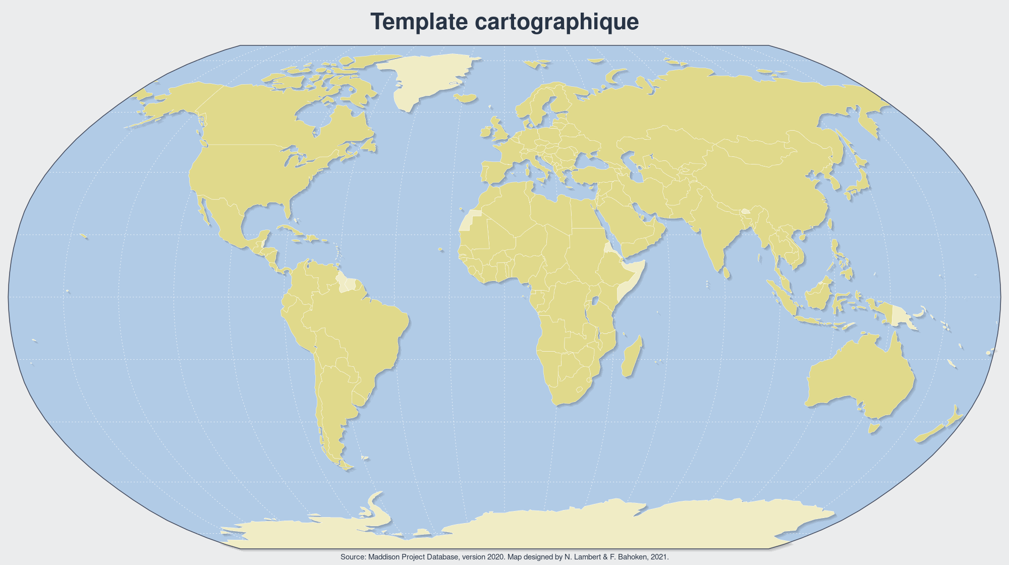
Centroïdes
drawcentroids <- function(var = "pop", year = 2018, col = red, r = 10,
                        title = "Map Title"){
x <- getcentroids(var, year)
circles <- st_buffer(sf::st_as_sf(x, coords =c('x', 'y'),
                                  crs = sf::st_crs(sphere)), dist = r)
template(year = year, title)
plot(st_geometry(circles), col = col, border= "#283445", lwd = 0.5, add= T)
}
file <- "maps/centroids.png"
if (!file.exists(file)){
png(file, width = 2000, height = 1120, res = 150)
drawcentroids(var = "pop",year = 2018, r = 75000, col = "black",
title = "Centroïdes des pays dont les données sont disponibles, 2018")
dev.off()
}png
2 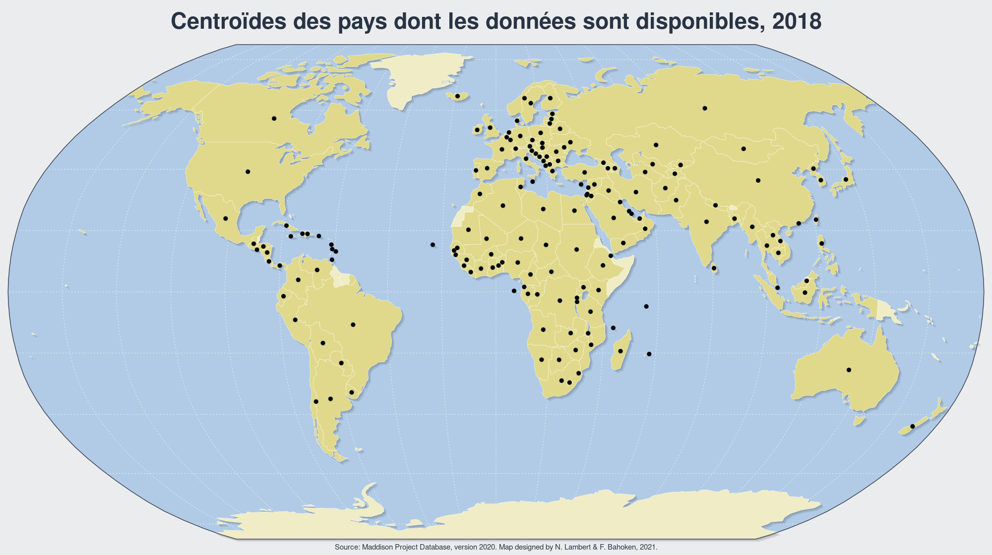
Symboles proportionnels
NB : Même si cela aurait été plus facile, le choix a été fait ici de ne pas utiliser le [package cartography] (https://cran.r-project.org/web/packages/cartography/index.html) afin d’exploiter au mieux les fonctionnalités de base de R. L’objectif est d’avoir une très grande comparabilité entre les cartes.
propsymbols <- function(var = "pop", year = 2018, k = 1, col = red,
                        title = "Map Title", leg.title = "Legend"){
x <- getcentroids(var, year)
x <- x[order(x$v, decreasing = TRUE),]
x$r <- sqrt(x$v * k)
circles <- st_buffer(sf::st_as_sf(x, coords =c('x', 'y'),
                                  crs = sf::st_crs(sphere)), dist = x$r)
template(year = year, title = title)
plot(st_geometry(circles), col = col, border= "#283445", lwd = 0.5, add= T)
legend(x = circles, var = "v", pos =c(-12000000,-5000000), title.txt = leg.title)
}
file <- "maps/propsymbolspop2018.png"
if (!file.exists(file)){
png(file, width = 2000, height = 1120, res = 150)
propsymbols(var = "pop",year = 2018, k = kpop, col = blue,
title = "Population mondiale par symboles proportionnels en 2018",
leg.title = "Population (en hab.)")
dev.off()
}png
2 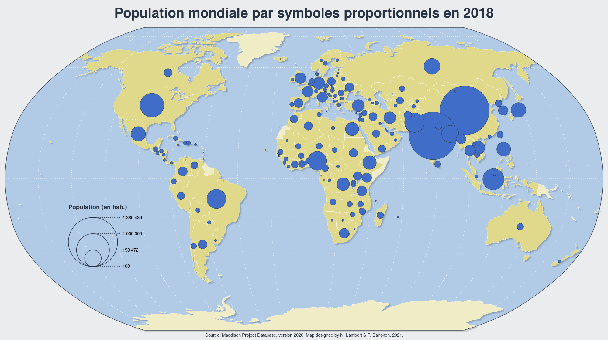
file <- "maps/propsymbolsgdp2018.png"

if (!file.exists(file)){
  png(file, width = 2000, height = 1120, res = 150)
  propsymbols(var = "gdp",year = 2018, k = kgdp, col = red,
            title = "PIB mondial par symboles proportionnels en 2018",
            leg.title = "PIB en milliards (US$ 2011)")
  dev.off()

}
png
2 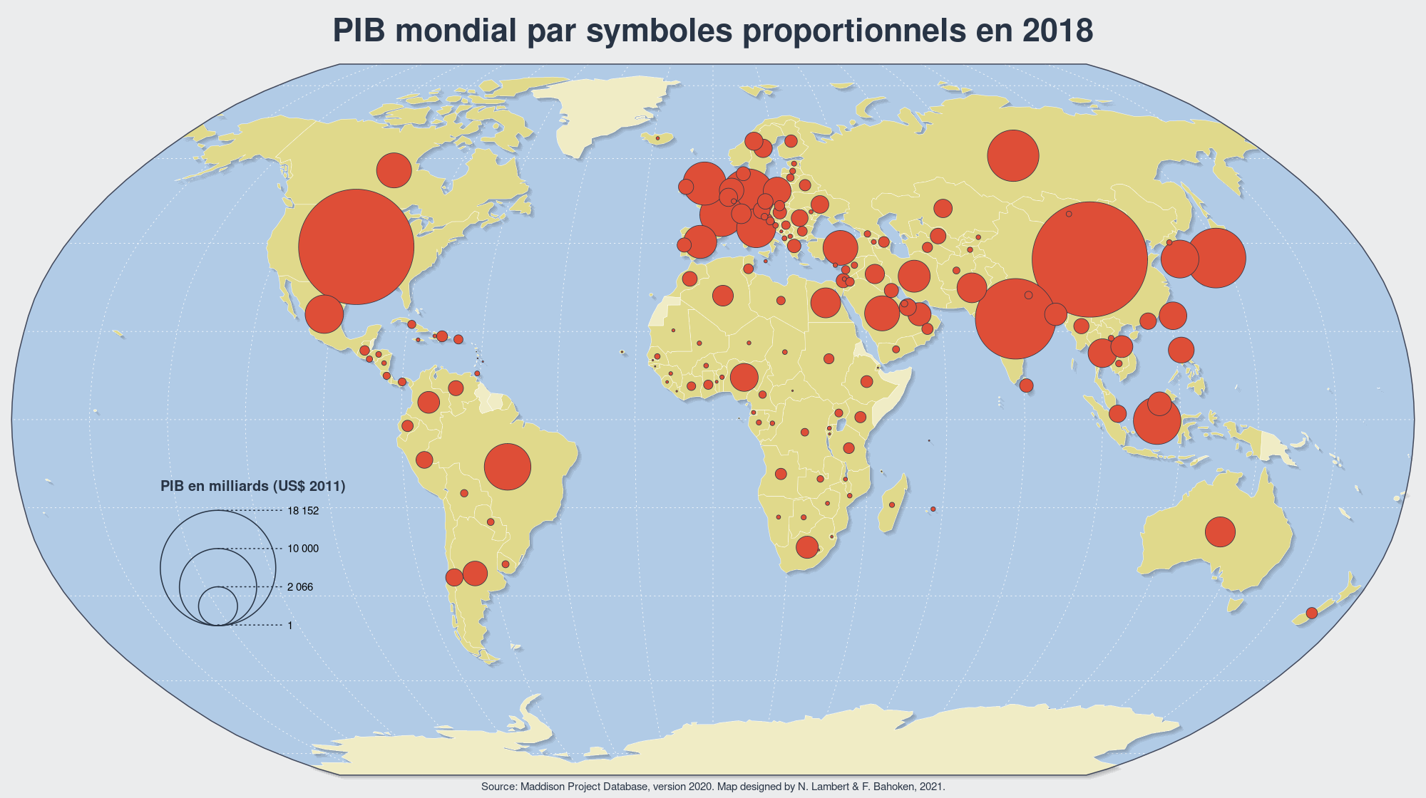
Carte par points
dotdensitymap <- function(var = "pop", year = 2018, onedot = 1, radius = 1,
                          col = red, title = "Map Title", unit =""){

if (year <= 1991){x <- world1}
if (year == 1992){x <- world2}
if (year >= 1993){x <- world3}
x <- merge(x, maddison[maddison$year == year,], by.x = "id",
           by.y = "countrycode")
x <- x[,c("id",var,"geometry")]
x[,"v"] <- round(x[,var] %>% st_drop_geometry() /onedot,0)
dots <- st_sample(x, x$v, type = "random", exact = TRUE)
circles <- st_buffer(dots, dist = radius)

template(year = year, title = title)
plot(st_geometry(circles), col = col, border= "#283445", lwd = 0.5, add = T)
text(x= 0, y = -6000000, paste0("1 point = ",onedot, " ",unit),
       cex = 1.1, pos = 3, font = 2, col = col)
}
file <- "maps/dotdensitypop2018.png"
if (!file.exists(file)){
png(file, width = 2000, height = 1120, res = 150)
dotdensitymap(var = "pop", year = 2018, onedot = 10000, radius = 100000,
col = blue, title = "Population mondiale, 2018", unit ="hab.")
dev.off()
}png
2 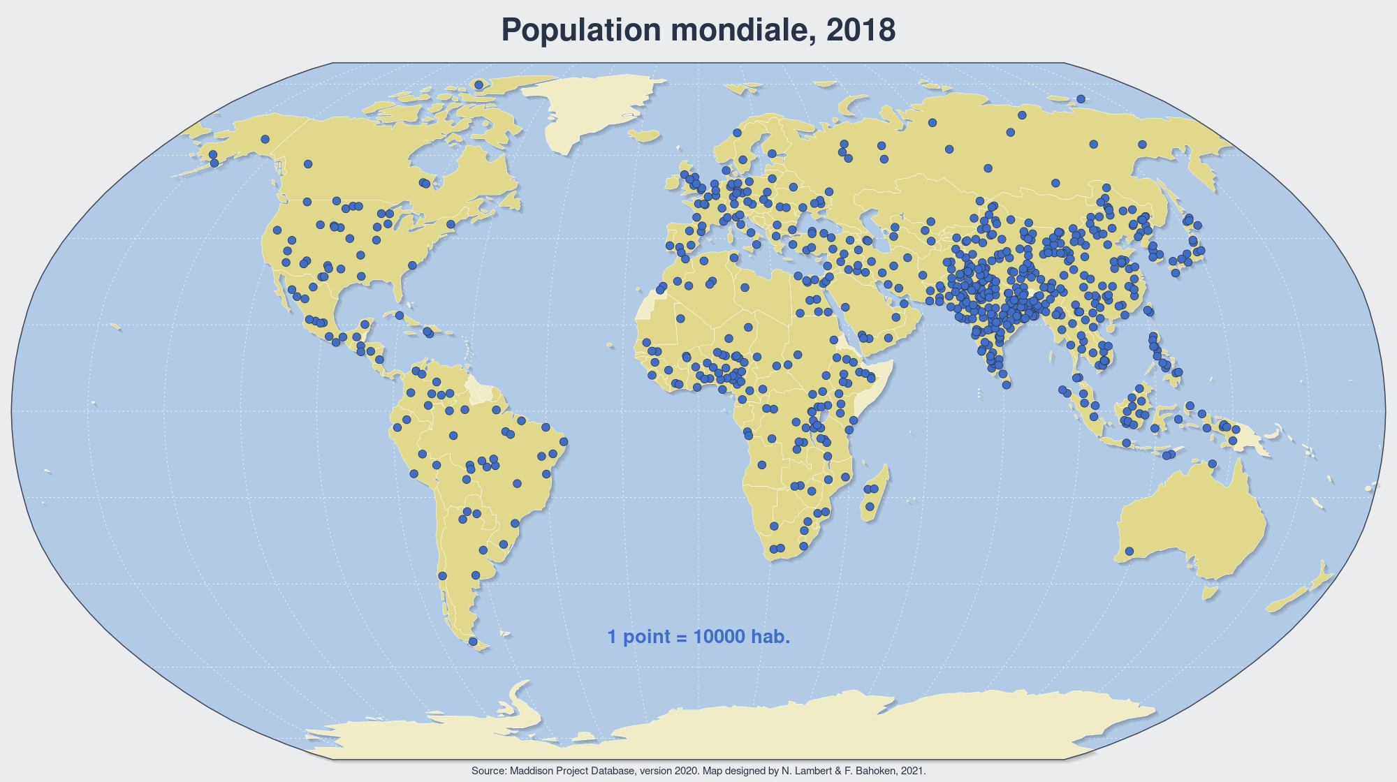
file <- "maps/dotdensitygdp2018.png"

if (!file.exists(file)){

png(file, width = 2000, height = 1120, res = 150)
dotdensitymap(var = "gdp", year = 2018, onedot = 100, radius = 100000,
                          col = red, title = "PIB mondial, 2018", unit ="milliards $")
dev.off()
}
png
2 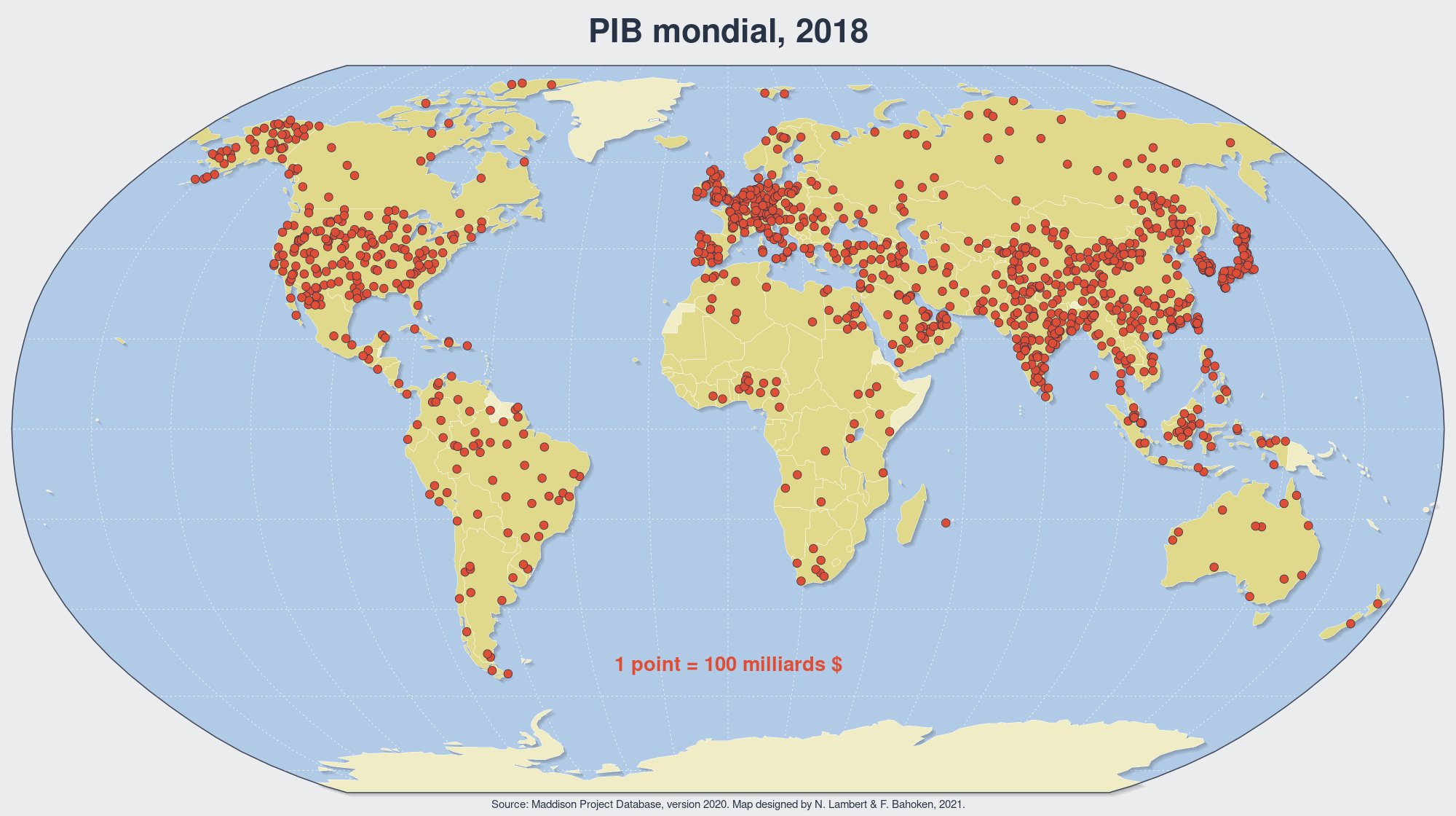
Cartogramme de Dorling
dorling <- function(var = "pop", year = 2018, k = 1, itermax = 10,
                    col = red, title = "Map Title", leg.title ="Legend"){

x <- getcentroids(var, year)

dat.init <- x[,c("x","y","v")]
dat.init$v <- sqrt(dat.init$v * k)
simulation <- circleRepelLayout(x = dat.init, xysizecols = 1:3,
                                wrap = FALSE, sizetype = "radius",
                                maxiter = itermax, weights =1)$layout
circles <- st_buffer(sf::st_as_sf(simulation, coords =c('x', 'y'),
                      crs = sf::st_crs(sphere)), dist = simulation$radius)
circles$v = x$v
template(year = year, title = title)
plot(st_geometry(circles), col = col, border= "#283445", lwd = 0.5, add= T)
legend(x = circles, var = "v", pos =c(-12000000,-5000000), title.txt = leg.title)
}
file <- "maps/drolingpop2018.png"
if (!file.exists(file)){
png(file, width = 2000, height = 1120, res = 150)
dorling(var = "pop",year = 2018, k = kpop, itermax = 10, col = blue,
title = "Population mondiale par cartogrammes de Dorling, 2018",
leg.title = "Population (en hab.)")
dev.off()
}png
2 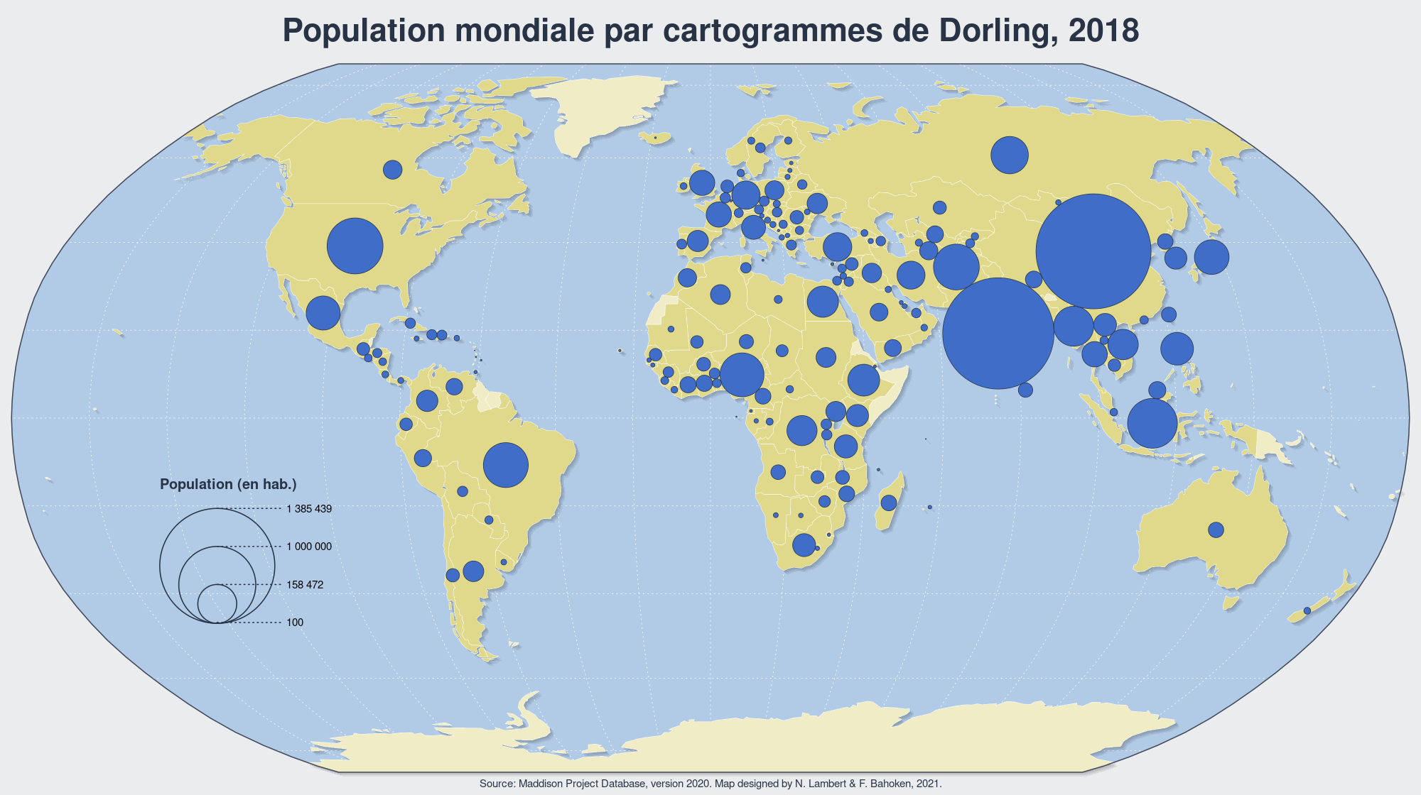
file <- "maps/drolinggdp2018.png"

if (!file.exists(file)){
  png(file, width = 2000, height = 1120, res = 150)
  dorling(var = "gdp",year = 2018, k = kgdp, itermax = 10, col = red,
            title = "Richesse mondiale par cartogrammes de Dorling Cartogram, 2018",
          leg.title = "PIB en milliards (2011 US$)")
  dev.off()

}
png
2 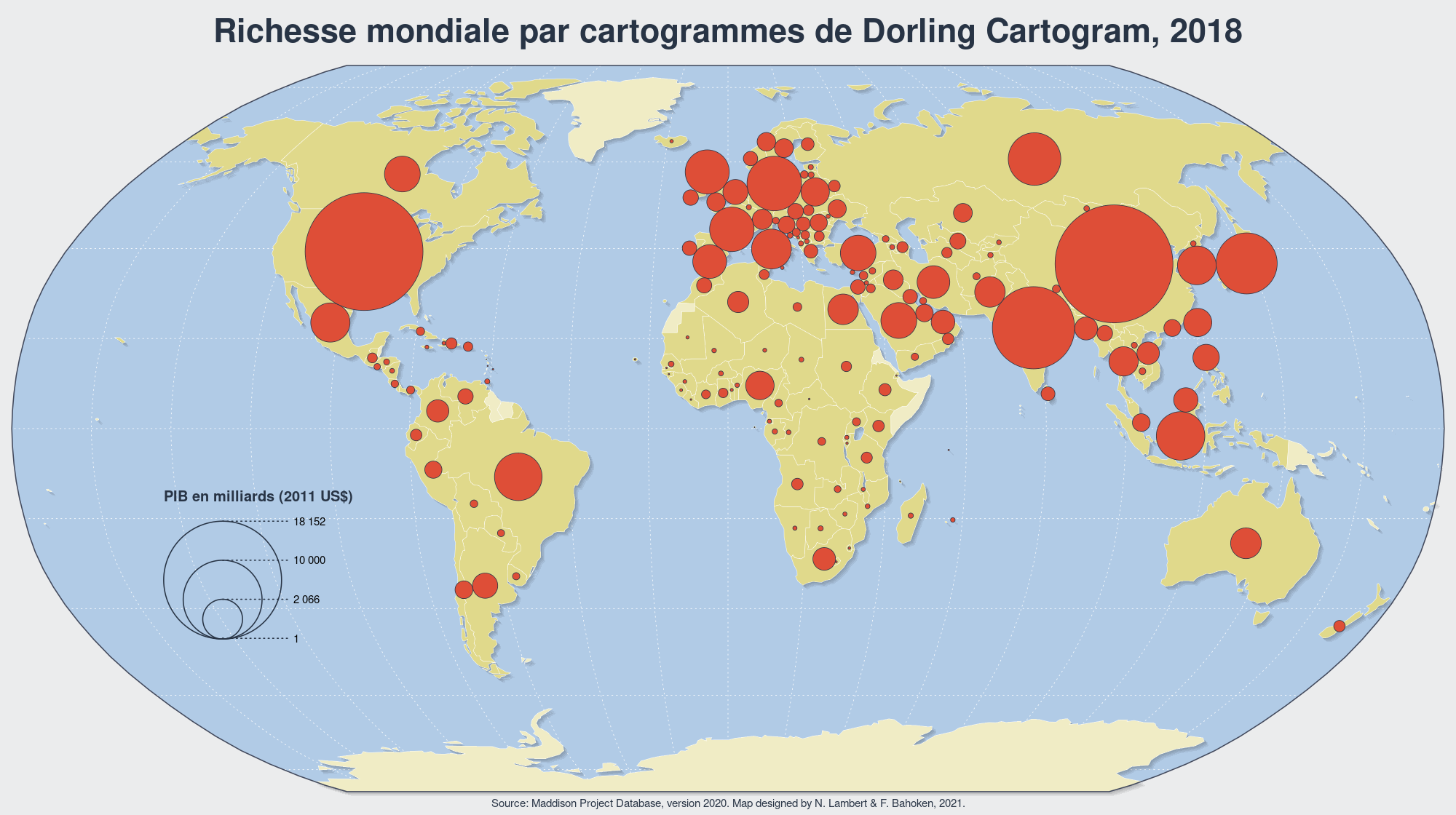
Cartogramme par points
dotcartogram <- function(var = "pop", year = 2018, itermax = 10,
                          onedot = 1, radius = 1, col = red,
                          title = "Map Title", unit = ""){

x <- getcentroids(var, year)
x$v <- round(x$v/onedot,0)
x <- x[x$v > 0,]

dots <- x[x$v == 1,c("x","y","v")]
rest <-  x[x$v  > 1,c("x","y","v")]

nb <- nrow(rest)
for (i in 1:nb){
  new <- rest[i,]
  new$v <- 1
  for (j in 1:rest$v[i]){ dots <- rbind(dots,new)}
}

dots$x <- jitter(dots$x)
dots$y <- jitter(dots$y)
dots$v <- radius

simulation <- circleRepelLayout(x = dots, xysizecols = 1:3,
                                wrap = FALSE, sizetype = "radius",
                                maxiter = itermax, weights =1)$layout
circles <- st_buffer(sf::st_as_sf(simulation, coords =c('x', 'y'),
                      crs = sf::st_crs(sphere)), dist = radius)
template(year = year, title = title)
plot(st_geometry(circles), col = col, border= "#283445", lwd = 0.5, add= T)
  text(x= 0, y = -6000000, paste0("1 point = ",onedot, " ",unit), cex = 1.1, pos = 3, font = 2,
       col = col)
}
file <- "maps/dotcartogrampop2018.png"
if (!file.exists(file)){
png(file, width = 2000, height = 1120, res = 150)
dotcartogram(var = "pop",year = 2018, itermax = 70, onedot = 10000,
radius = 100000, col = blue,
title = "Cartogramme par points de la population mondiale en 2018", unit = "hab.")
dev.off()
}png
2 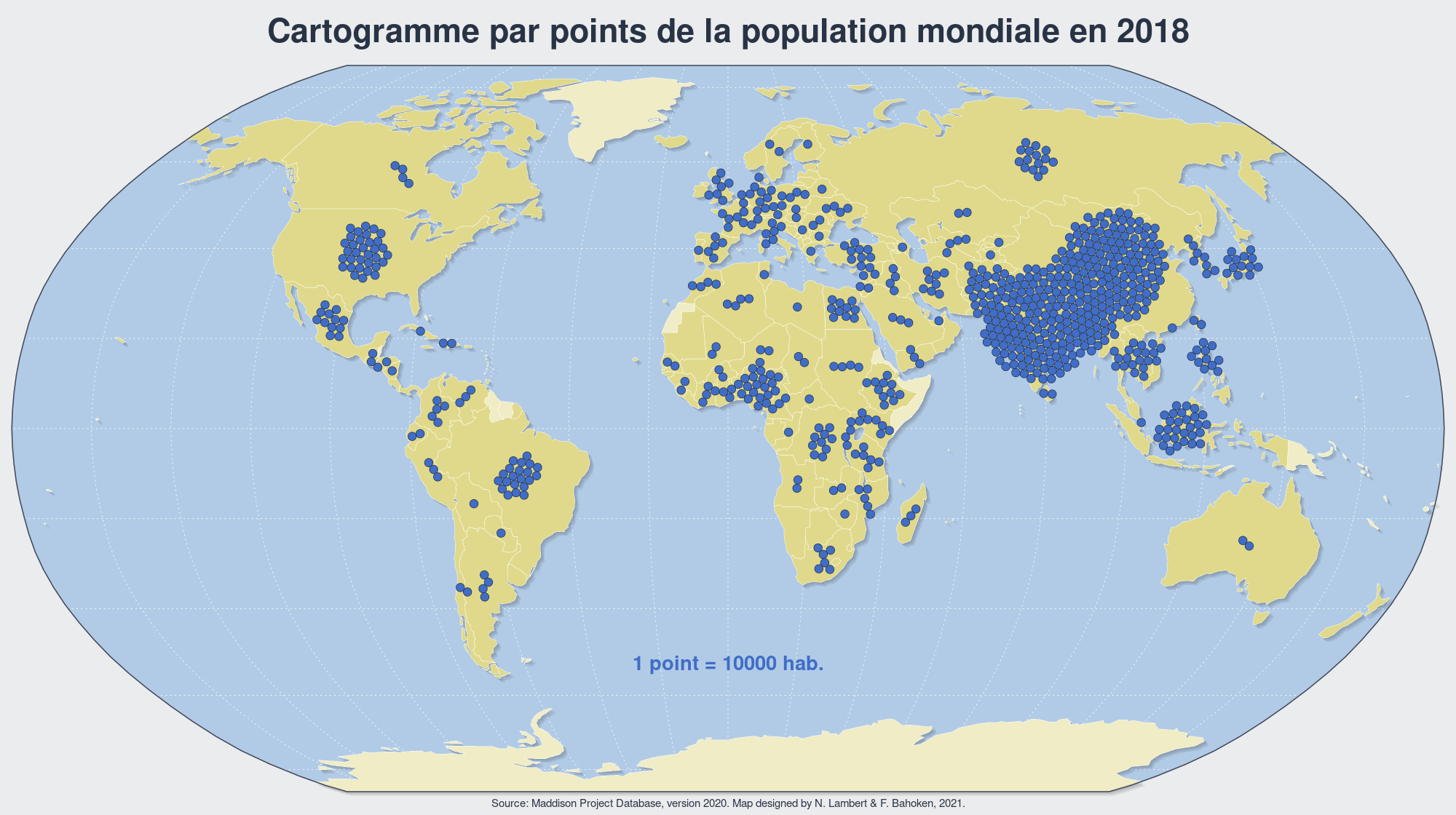
file <- "maps/dotcartogramgdp2018.png"

if (!file.exists(file)){
  png(file, width = 2000, height = 1120, res = 150)
  dotcartogram(var = "gdp",year = 2018, itermax = 70, onedot = 100,
                radius = 100000, col = red,
                title = "Dodge Dotmap du PIB mondial en 2018",  unit = "milliards $")
  dev.off()

}
png
2 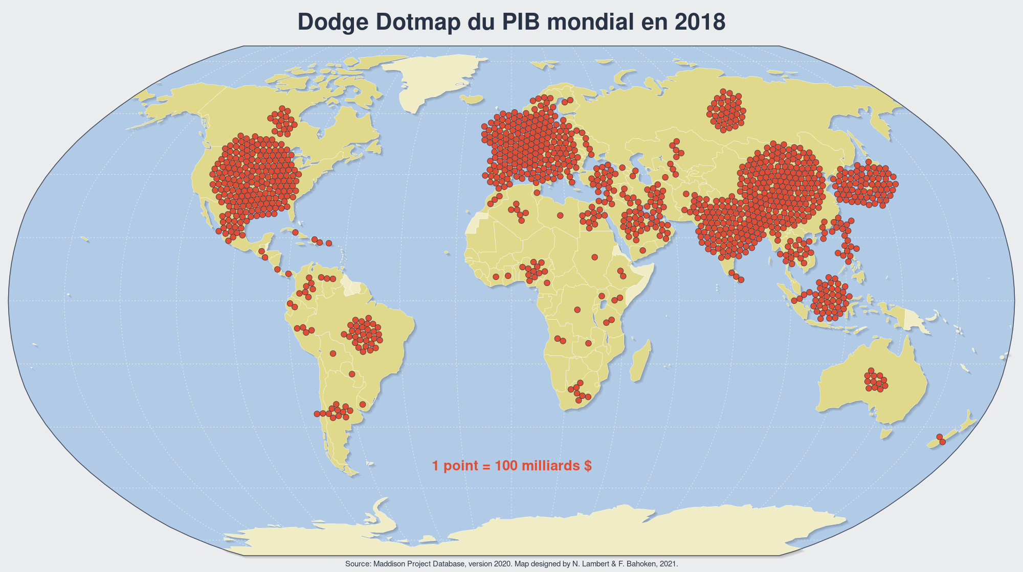
Bien sûr, nous pouvons modifier la taille et la valeur de chaque point.
file <- "maps/dotcartogramgdp2018_v2.png"

if (!file.exists(file)){
  png(file, width = 2000, height = 1120, res = 150)
  dotcartogram(var = "gdp",year = 2018, itermax = 100, onedot = 20,
                radius = 60000, col = red,
                title = "Cartogramme par points du PIB mondial, 2018", unit = "milliards de $")
  dev.off()

}
png
2 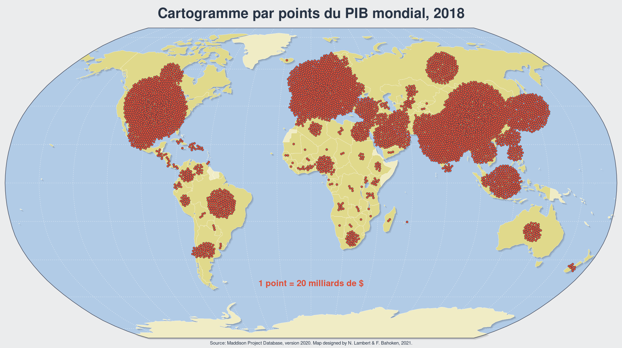
Cartogramme par points (amélioration)
Ici, nous ajoutons le paramètre “position” à la fonction dotcartogram afin que les points puissent être disposés de manière régulière ou aléatoire à l’intérieur des pays, et non plus seulement répartis à partir du centroïde. Les trois cartes suivantes vous permettent de visualiser l’effet de ce paramètre.
dotcartogram2 <- function(var = "pop", year = 2018, itermax = 10,
                          onedot = 1, position = "center", radius = 1, col = red,
                          title = "Map Title", unit = ""){

if (position %in% c("regular","random")){
if (year <= 1991){x <- world1}
if (year == 1992){x <- world2}
if (year >= 1993){x <- world3}
x <- merge(x, maddison[maddison$year == year,], by.x = "id",
           by.y = "countrycode")
x <- x[,c("id",var,"geometry")]
x[,"v"] <- round(x[,var] %>% st_drop_geometry() /onedot,0)
x = x[x$v > 0,]
dots <- st_sample(x, x$v, type = position, exact = TRUE)
dots <- data.frame(st_coordinates(dots),radius)
colnames(dots) <- c("x","y","v")
}

if (position == "center"){

  x <- getcentroids(var, year)
x$v <- round(x$v/onedot,0)
x <- x[x$v > 0,]

dots <- x[x$v == 1,c("x","y","v")]
rest <-  x[x$v  > 1,c("x","y","v")]

nb <- nrow(rest)
for (i in 1:nb){
  new <- rest[i,]
  new$v <- 1
  for (j in 1:rest$v[i]){ dots <- rbind(dots,new)}
}

dots$x <- jitter(dots$x)
dots$y <- jitter(dots$y)
dots$v <- radius

}

simulation <- circleRepelLayout(x = dots, xysizecols = 1:3,
                                wrap = FALSE, sizetype = "radius",
                                maxiter = itermax, weights =1)$layout
circles <- st_buffer(sf::st_as_sf(simulation, coords =c('x', 'y'),
                      crs = sf::st_crs(sphere)), dist = radius)


template(year = year, title = title)
plot(st_geometry(circles), col = col, border= "#283445", lwd = 0.5, add= T)
text(x= 0, y = -6000000, paste0("1 point = ",onedot, " ",unit), cex = 1.1, pos = 3, font = 2,
       col = col)

}
Position = “center”
file <- "maps/center_dotcartogramgdp2018.png"

if (!file.exists(file)){
  png(file, width = 2000, height = 1120, res = 150)
  dotcartogram2(var = "gdp",year = 2018, itermax = 100, onedot = 60,
                radius = 80000, col = red,
                position = "center",
                title = "Cartogramme par points du PIB (centre)",
                unit = "milliards de $")
  dev.off()

}
png
2 
Carte avec position = “random”
file <- "maps/random_dotcartogramgdp2018.png"

if (!file.exists(file)){
  png(file, width = 2000, height = 1120, res = 150)
  dotcartogram2(var = "gdp",year = 2018, itermax = 100, onedot = 60,
                radius = 80000, col = red,
                position = "random",
                title = "Cartogramme par points du PIB (aléatoire)",
                unit = "milliards de $")
  dev.off()

}
png
2 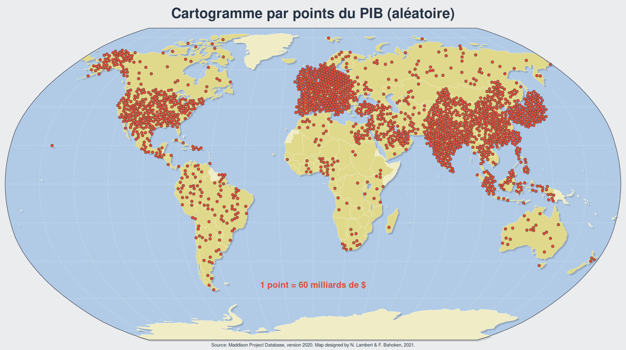
Position = “regular”
file <- "maps/regular_dotcartogramgdp2018.png"

if (!file.exists(file)){
  png(file, width = 2000, height = 1120, res = 150)
  dotcartogram2(var = "gdp",year = 2018, itermax = 100, onedot = 60,
                radius = 80000, col = red,
                position = "regular",
                title = "Cartogramme par points du PIB (régulier)",
                unit = "milliards de $")
  dev.off()
}
png
2 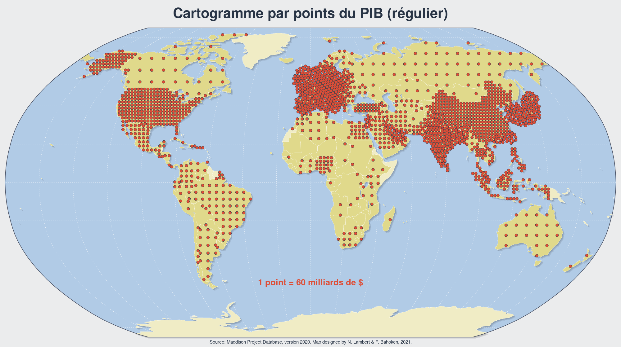
Variation 1
Dans cette variante, nous proposons de colorer les points en fonction d’une donnée quantitative relative : le pib par habitant. Pour faire simple, et parce que ce point particulier n’est pas central ici, nous utilisons dans ce cas le package mapsf.
library(mapsf)

var = "gdp"
year = 2018
itermax = 100
onedot = 50
radius = 90000
cols <- c("#ffffb2","#fed976","#feb24c","#fd8d3c","#f03b20","#bd0026")
title = "La richesse dans le monde en 2018"
unit = "milliards de $"
file <- "maps/dodgeratio.png"


if (!file.exists(file)){

  x <- getcentroids(var, year)
  x$v <- round(x$v/onedot,0)
  x <- x[x$v > 0,]

  x <- merge(x, maddison[maddison$year == year,], by.x = "id", by.y = "countrycode")
  x <- x[,c("x","y","v","gdppc")]
  colnames(x) <- c("x","y","v","s")
  dots <- x[x$v == 1,c("x","y","v","s")]
  rest <-  x[x$v  > 1,c("x","y","v","s")]
  nb <- nrow(rest)
  for (i in 1:nb){
    new <- rest[i,]
    new$v <- 1
    for (j in 1:rest$v[i]){ dots <- rbind(dots,new)}
  }

  dots$x <- jitter(dots$x)
  dots$y <- jitter(dots$y)
  dots$v <- radius

  simulation <- circleRepelLayout(x = dots, xysizecols = 1:3,
                                  wrap = FALSE, sizetype = "radius",
                                  maxiter = itermax, weights =1)$layout
  simulation$s <- dots$s

  circles <- st_buffer(sf::st_as_sf(simulation, coords =c('x', 'y'),
                        crs = sf::st_crs(sphere)), dist = radius)

  png(file, width = 2000, height = 1120, res = 150)
  template(year = year, title = title)

  mf_map(x = circles, var = "s", type = "choro",   pal = cols,
  breaks = "quantile", nbreaks = 6, leg_val_rnd = 0,
  leg_pos = c(-13000000, -1000000), leg_title = "PIB par habitant (en $)",
  add = TRUE)

  text(x= 0, y = -6000000, paste0("1 point = ",onedot, " ",unit), cex = 1.1, pos = 3, font = 2,
         col = red)

  dev.off()
}
png
2 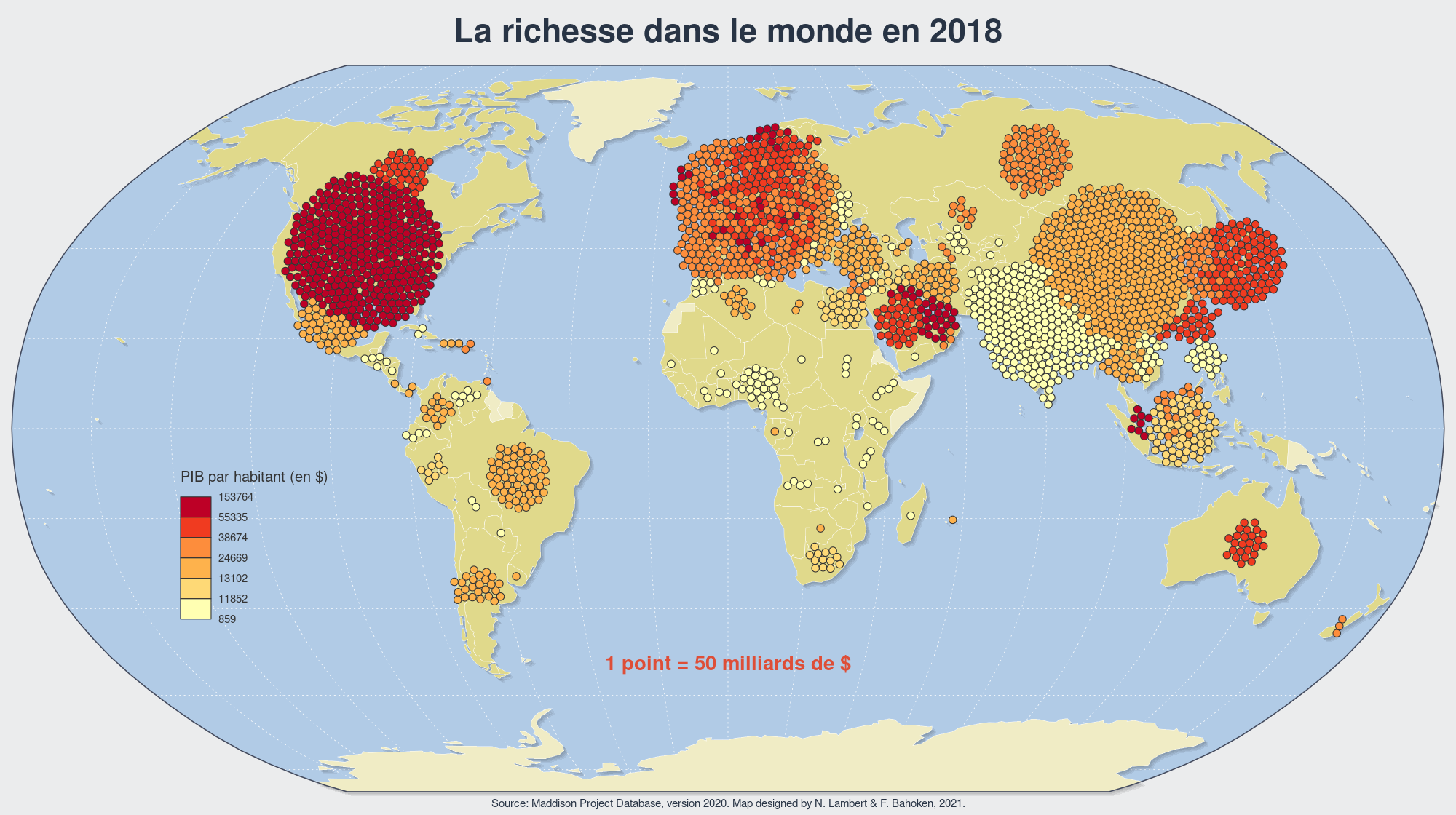
Variation 2
Ici, nous proposons une autre alternative où le nombre de points dans chaque pays est le même. C’est le paramètre qui est fixé. Par conséquent, la surface des cercles à l’intérieur des pays est modifiée pour refléter les quantités. Ci-dessous, nous décidons d’avoir 50 points par pays.
dotcartogram4 <- function(var = "pop", year = 2018, itermax = 10,
                          divide = 4, k = 1, col = red,
                          title = "Map Title", legtitle = "Legend"){

x <- getcentroids(var, year)
x <- x[x$v > 0,c("x","y","v")]

dots <- x
for (i in 1:(round(divide) - 1)){
  dots <- rbind(dots,x)
}

dots$x <- jitter(dots$x)
dots$y <- jitter(dots$y)
dots$v <- sqrt(dots$v/divide * k)

simulation <- circleRepelLayout(x = dots, xysizecols = 1:3,
                                wrap = FALSE, sizetype = "radius",
                                maxiter = itermax, weights =1)$layout
circles <- st_buffer(sf::st_as_sf(simulation, coords =c('x', 'y'),
                      crs = sf::st_crs(sphere)), dist = simulation$radius)

#legend(x = circles, var = "v", pos =c(-12000000,-5000000), title.txt = legtitle)
template(year = year, title = title)
plot(st_geometry(circles), col = col, border= "#283445", lwd = 0.5, add= T)
}
file <- "maps/dotcartogrampop2018_alter.png"
if (!file.exists(file)){
png(file, width = 2000, height = 1120, res = 150)
dotcartogram4(var = "pop",year = 2018, k = kpop, itermax = 20, divide = 50, col = blue,
title = "Population mondiale, en 2018 (divide = 50)", legtitle = "Nombre d'habitants")
dev.off()
}png
2 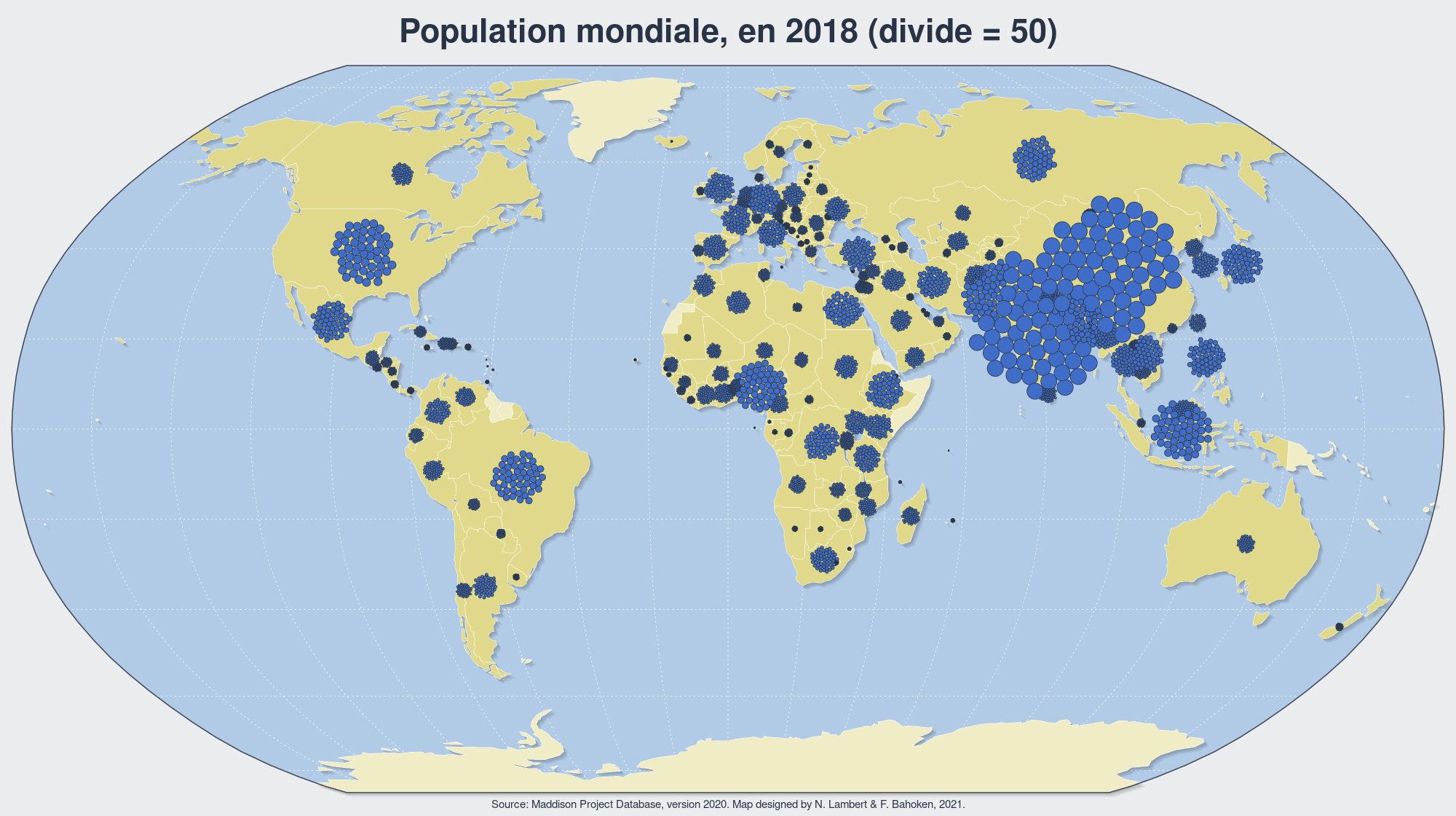
file <- "maps/dotcartogramgdp2018_alter.png"

if (!file.exists(file)){
  png(file, width = 2000, height = 1120, res = 150)
  dotcartogram4(var = "gdp",year = 2018, k = kgdp, itermax = 20, divide = 50, col = red,
            title = "PIB mondial en 2018 (divide = 50)", legtitle = "PIB (en $)")
  dev.off()

}
png
2 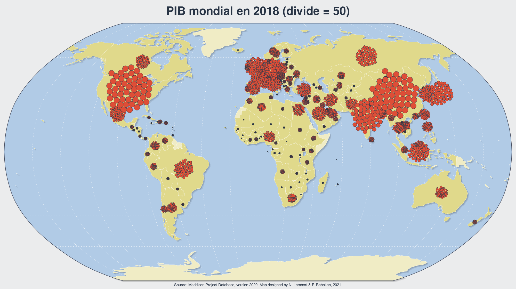
Timelines
PIB de 1950 à 2018.
for (year in 1950:2018){

file <- paste0("tmp/gdp/gdp_",year,".png" )

if (!file.exists(file)){
   png(file, width = 2000, height = 1120, res = 150)
   dotcartogram(var = "gdp",year = year, itermax = 100, onedot = 40,
                 radius = 75000, col = red,
                 title = paste0("Richesse mondiale en ", year), unit = "milliards de $")
   dev.off()

}

}
png -> gif
file <- "maps/gdp.gif"
if (!file.exists(file)){
frames <- paste0("tmp/gdp/",list.files("tmp/gdp"))
m <- image_read(frames)
m <- image_animate(m)
image_write(m, file)
}
Population de 1950 à 2018.
for (year in 1950:2018){

file <- paste0("tmp/pop/pop_",year,".png" )

if (!file.exists(file)){
   png(file, width = 2000, height = 1120, res = 150)
   dotcartogram(var = "pop",year = year, itermax = 100, onedot = 4000,
                 radius = 75000, col = blue,
                 title = paste0("Population mondiale en ", year), unit = "hab.")
   dev.off()

}

}
png -> gif
file <- "maps/pop.gif"
if (!file.exists(file)){
frames <- paste0("tmp/pop/",list.files("tmp/pop"))
m <- image_read(frames)
m <- image_animate(m)
image_write(m, file)
}
Comparaison Dorling / Cartogramme par points
file <- "maps/pop_transform.gif"
if (!file.exists(file)){
frames <- c("maps/drolingpop2018.png", "maps/dotcartogrampop2018.png")
m <- image_read(frames)
m <- image_animate(m, fps = 2)
image_write(m, file)
}![]()
file <- "maps/gdp_transform.gif"
if (!file.exists(file)){
frames <- c("maps/drolinggdp2018.png","maps/dotcartogramgdp2018.png")
m <- image_read(frames)
m <- image_animate(m, fps = 2)
image_write(m, file)
}![]()
Addendum
La méthode est également disponible en javascript avec la bibliothèque D3.js. Le code est disponible ici et le résultat est affiché ci-dessous.
La méthode est également implémentée dans la bibliothèque JavaScript bertin. Voir : @neocartocnrs/bertin-js-dots-cartograms